# packages
library(galah)
library(ggplot2)
library(dplyr)
library(sf)
library(ozmaps)
library(tidyr)
library(stringr)
galah_config(email = "your-email-here") # ALA-registered email

desert_plant <- galah_call() |>
  filter(doi == "https://doi.org/10.26197/ala.0ef34e25-211f-4a8b-8237-db9cc169a272") |>
  atlas_occurrences()

frogs <- galah_call() |>
  filter(doi == "https://doi.org/10.26197/ala.1bd3f8b0-f17c-4411-a1ef-280ceb6c991b") |>
  atlas_occurrences()

native_mice <- galah_call() |>
  filter(doi == "https://doi.org/10.26197/ala.3cbcf19d-2df3-480f-b6ad-2fb1fa8a0f65") |>
  atlas_occurrences()

acacias <- galah_call() |>
  filter(doi == "https://doi.org/10.26197/ala.ace35c33-584e-4b9b-a12c-53f6f37cd1ab") |>
  atlas_occurrences()

butterflies <- galah_call() |>
  filter(doi == "https://doi.org/10.26197/ala.1b1d1c75-1395-4ce1-bbc0-80bb7574a0f3") |>
  atlas_occurrences()

bitter_peas <- galah_call() |>
  filter(doi == "https://doi.org/10.26197/ala.575871f9-e687-442f-bf05-065e2a8c5811") |>
atlas_occurrences()10 Geospatial cleaning
Geospatial observational data provide essential information about species’ locations over time and space, and can be combined with ecological data to understand species-environment interactions. However, working with geospatial data can be challenging, as seemingly minor issues can significantly impact data validity.
Outliers—data points that are considerably distant from the majority of a species’ observations and can skew overall distribution—are a major challenge in geospatial data cleaning. Identifying outliers can be difficult because it’s not always clear whether they are true outliers or data errors. Errors can result from species misidentification or incorrect geo-referencing. Other accidental errors, such as reversing numeric symbols, mistyping coordinates, or entering incorrect locations, can dramatically affect the reported location of a species. For species with smaller ranges, these errors may be easier to detect. However, for species with larger ranges or analyses involving many species over a large area, these errors become much more difficult to identify.
Every dataset has its own combination of issues requiring bespoke cleaning methods (e.g. (Jin and Yang 2020)). It is crucial to clean geospatial data effectively to ensure their usefulness, as errors can lead to unexpected results in species range estimates and analytic outputs.
In this chapter, we will highlight common issues with coordinate data and demonstrate how to correct or remove suspicious-seeming records.
TipChecklist
This chapter can be read more like a checklist of possible geospatial errors in a dataset, how to identify them, and how to fix them.
10.0.1 Prerequisites
In this chapter we’ll use several datasets:
- MacDonnell’s desert fuschia (Eremophila macdonnellii) occurrence records from the ALA
- Red-eyed tree frog (Litoria chloris) occurrence records in 2013 from the ALA
- Kowari (Dasyuroides byrnei, a native mouse) occurrence records from the ALA
- Acacia occurrence records from the ALA
- Common brown butterfly (Heteronympha merope) occurrence records in 2014 from the ALA
- Bitter pea (Daviesia ulicifolia) occurrence records from the ALA


10.1 Missing coordinates
As discussed in Missing Values chapter, many spatial analytical tools are not compatible with missing coordinate data. We recommend identifying the rows that have missing data before deciding to exclude them.
# Identify missing data in coordinates
desert_plant |>
  filter(is.na(decimalLatitude) | is.na (decimalLongitude))
# A tibble: 95 × 9
recordID scientificName taxonConceptID decimalLatitude decimalLongitude
<chr> <chr> <chr> <dbl> <dbl>
1 000d4874-8c74… Eremophila ma… https://id.bi… NA NA
2 050653b6-a41c… Eremophila ma… https://id.bi… NA NA
3 06e69581-7d6d… Eremophila ma… https://id.bi… NA NA
4 0973271a-e222… Eremophila ma… https://id.bi… NA NA
5 0eead38f-0c16… Eremophila ma… https://id.bi… NA NA
6 0f52e34b-a803… Eremophila ma… https://id.bi… NA NA
7 1185c4f9-1cb6… Eremophila ma… https://id.bi… NA NA
8 1190b3b9-90d8… Eremophila ma… https://id.bi… NA NA
9 13a24c07-f628… Eremophila ma… https://id.bi… NA NA
10 18d11ae3-e558… Eremophila ma… https://id.bi… NA NA
# ℹ 85 more rows
# ℹ 4 more variables: eventDate <dttm>, occurrenceStatus <chr>,
# dataResourceName <chr>, PRESUMED_SWAPPED_COORDINATE <lgl>You can use drop_na() to remove missing values from your dataset.
# Excluding them
desert_plant <- desert_plant |>
tidyr::drop_na(decimalLatitude, decimalLongitude)- 1
-
You could also use
filter(!is.na(decimalLatitude), !is.na(decimalLongitude))to achieve the same thing
10.2 Correcting fixable coordinate errors
Spatial outliers can sometimes result from taxonomic misidentification, but not always. Occasionally, records that appear as outliers are true observations of a species but contain mistakes in their coordinates. To avoid unnecessarily deleting data, it’s good practice to use multiple sources of spatial information to decide whether an unexpected data point is due to a small but fixable error in coordinates.
Many coordinate issues can be solved through data manipulation rather than discarding the data. Here are several coordinate issues that can be identified and corrected.
10.2.1 Swapped numeric sign
If you notice a cluster of points mirrored in the opposite hemisphere, consider correcting the sign instead of discarding the points.
Let’s use MacDonnell’s desert fuschia occurrence records for our example. Including the PRESUMED_SWAPPED_COORDINATE assertion column when downloading records using the galah package allows us to identify records flagged as potentially having swapped coordinates.
desert_plant <- desert_plant |>
  drop_na(decimalLongitude, decimalLatitude) # remove NA coordinates

desert_plant |>
  select(PRESUMED_SWAPPED_COORDINATE, everything())
# A tibble: 930 × 9
PRESUMED_SWAPPED_COO…¹ recordID scientificName taxonConceptID decimalLatitude
<lgl> <chr> <chr> <chr> <dbl>
1 FALSE 0009009… Eremophila ma… https://id.bi… -22.8
2 FALSE 002e372… Eremophila ma… https://id.bi… -25.3
3 FALSE 0034dc0… Eremophila ma… https://id.bi… -23.9
4 FALSE 0063223… Eremophila ma… https://id.bi… -24.5
5 FALSE 00d15a5… Eremophila ma… https://id.bi… -27.8
6 FALSE 013049a… Eremophila ma… https://id.bi… -25.2
7 FALSE 015571a… Eremophila ma… https://id.bi… -22.1
8 FALSE 01b5e44… Eremophila ma… https://id.bi… -25.2
9 FALSE 02524e1… Eremophila ma… https://id.bi… -25.1
10 FALSE 026c225… Eremophila ma… https://id.bi… -25.8
# ℹ 920 more rows
# ℹ abbreviated name: ¹PRESUMED_SWAPPED_COORDINATE
# ℹ 4 more variables: decimalLongitude <dbl>, eventDate <dttm>,
# occurrenceStatus <chr>, dataResourceName <chr>If we plot these records on a map and colour the points based on values in the PRESUMED_SWAPPED_COORDINATE assertion column, we can see that there is a single record (in orange) that looks like its coordinates have been mirrored across hemispheres.
# Retrieve map of Australia
aus <- st_transform(ozmap_country, 4326)

ggplot() +
  geom_sf(data = aus) +
  geom_point(data = desert_plant,
             aes(x = decimalLongitude,
                 y = decimalLatitude,
                 colour = PRESUMED_SWAPPED_COORDINATE)) +
  pilot::scale_color_pilot()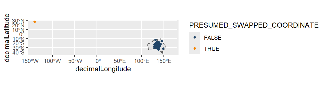
We can correct the numeric signs using if_else() from dplyr. The first statement updates our decimalLongitude column so that when decimalLongitude is less than 0, we remove the negative symbol by multiplying by -1, otherwise we keep the original longitude value. The second statement updates our decimalLatitude column using the same process.
desert_plant_filtered <- desert_plant |>
  mutate(
    decimalLongitude = if_else(decimalLongitude < 0,
      decimalLongitude * -1,
      decimalLongitude
    ),
    decimalLatitude = if_else(decimalLatitude > 0,
      decimalLatitude * -1,
      decimalLatitude
    )
  )
And here’s the updated map, with the corrected coordinates.
ggplot() +
  geom_sf(data = aus) +
  geom_point(data = desert_plant_filtered,
             aes(x = decimalLongitude,
                 y = decimalLatitude,
                 colour = PRESUMED_SWAPPED_COORDINATE)) +
  pilot::scale_color_pilot()
10.2.2 Location description doesn’t match coordinates
Misalignment between location metadata and coordinates could indicate errors in the dataset, but it’s sometimes possible to rectify these. Let’s use red-eyed tree frog data as an example.
frogs <- frogs |>
  drop_na(decimalLatitude, decimalLongitude) # remove NA values

frogs
# A tibble: 25 × 14
recordID scientificName taxonConceptID decimalLatitude decimalLongitude
<chr> <chr> <chr> <dbl> <dbl>
1 0bbcdc4a-5638… Litoria chlor… https://biodi… -28.4 153.
2 16ecde94-6b9b… Litoria chlor… https://biodi… -28.4 153.
3 2ba9c818-e81a… Litoria chlor… https://biodi… -27.4 152.
4 4a1b77fa-3538… Litoria chlor… https://biodi… -30.1 153.
5 4d3274a4-f9cd… Litoria chlor… https://biodi… -27.4 153.
6 52c1043c-5f79… Litoria chlor… https://biodi… -29.7 152.
7 52d5551a-816d… Litoria chlor… https://biodi… -29.9 153.
8 5c2c4fb6-5c5f… Litoria chlor… https://biodi… -29.7 152.
9 5d4be730-cc39… Litoria chlor… https://biodi… -28.4 153.
10 73a3b671-13a7… Litoria chlor… https://biodi… -26.6 153.
# ℹ 15 more rows
# ℹ 9 more variables: eventDate <dttm>, occurrenceStatus <chr>,
# dataResourceName <chr>, countryCode <chr>, locality <chr>, family <chr>,
# genus <chr>, species <chr>, cl22 <chr>When we plot the coordinates of our red-eyed tree frog occurrences, there is an unexpected observation near Japan (or where Japan would appear if we had plotted more countries and not just Australia). This is quite surprising—red-eyed tree frogs are not native to Japan!
# Get a map of aus, transform projection
aus <- st_transform(ozmap_country, 4326)

# Map
ggplot() +
  geom_sf(data = aus,
          colour = "grey60") +
  geom_point(data = frogs,
             aes(x = decimalLongitude,
                 y = decimalLatitude),
             colour = "#557755")
Let’s check the countryCode column to see whether this might be an Australian record with a mistake in the coordinates. Using distinct(), we can see that there are 2 country codes…
frogs |>
  distinct(countryCode)
# A tibble: 2 × 1
countryCode
<chr>
1 AU
2 JP …and filtering to Japan ("JP") identifies our stray data point.
frogs |>
  filter(countryCode == "JP")
# A tibble: 1 × 14
recordID scientificName taxonConceptID decimalLatitude decimalLongitude
<chr> <chr> <chr> <dbl> <dbl>
1 c08e641e-cf01-… Litoria chlor… https://biodi… 24.5 152.
# ℹ 9 more variables: eventDate <dttm>, occurrenceStatus <chr>,
# dataResourceName <chr>, countryCode <chr>, locality <chr>, family <chr>,
# genus <chr>, species <chr>, cl22 <chr>So far this observation does seem to be in Japan. To be extra certain, we can also use the column locality, which provides additional information from the data collector about the record’s location.
frogs |>
  filter(countryCode == "JP") |>
  select(countryCode, locality, scientificName, decimalLatitude, decimalLongitude)
# A tibble: 1 × 5
countryCode locality scientificName decimalLatitude decimalLongitude
<chr> <chr> <chr> <dbl> <dbl>
1 JP mt bucca Litoria chloris 24.5 152.The locality column reveals the observation was made in “mt bucca”. This is surprising to see because Mt Bucca is a mountain in Queensland!
When we look at our Japan data point’s decimalLongitude and decimalLatitude alongside other values in our data, it becomes clear that the Japan data point seems to sit within the same numerical range as other points, but the decimalLatitude is positive rather than negative.
frogs |>
  arrange(desc(countryCode)) |>
  select(countryCode, decimalLongitude, decimalLatitude) |>
  print(n = 5)
# A tibble: 25 × 3
countryCode decimalLongitude decimalLatitude
<chr> <dbl> <dbl>
1 JP 152. 24.5
2 AU 153. -28.4
3 AU 153. -28.4
4 AU 152. -27.4
5 AU 153. -30.1
# ℹ 20 more rowsAll of this evidence suggests that our Japan “outlier” might instead be an occurrence point with a mis-entered latitude coordinate.
Let’s fix this by adding a negative symbol (-) to the record’s latitude coordinate number. We’ll use case_when() from dplyr to specify that if the countryCode == "JP", then we’ll multiply the decimalLatitude by -1, reversing the symbol.
frogs_fixed <- frogs |>
  mutate(
    decimalLatitude = case_when(
      countryCode == "JP" ~ decimalLatitude * -1,
      .default = decimalLatitude
    ))

frogs_fixed |>
  filter(countryCode == "JP") |>
  select(decimalLatitude, decimalLongitude, countryCode)
# A tibble: 1 × 3
decimalLatitude decimalLongitude countryCode
<dbl> <dbl> <chr>
1 -24.5 152. JP Mapping our data again shows our outlier is an outlier no longer!
Code
ggplot() +
  geom_sf(data = aus,
          colour = "grey60") +
  geom_point(data = frogs_fixed,
             aes(x = decimalLongitude,
                 y = decimalLatitude),
             colour = "#557755")
10.3 Excluding unfixable coordinate errors
Some coordinates issues cannot be fixed or inferred. In this case, it is important that you identify which records have issues and remove them prior to analysis. Here are some examples of geospatial errors that might need to be identified and removed in your dataset.
10.3.1 Flipped coordinates
Records with flipped coordinates typically appear as a group of points in an unexpected location. Although sometimes they can be fixed, this is not always the case.
Let’s use occurrence records of Kowari (a native, carnivorous mouse species) as an example. Including the COUNTRY_COORDINATE_MISMATCH assertion column when downloading records using the galah package allows us to identify records flagged as having mismatches between coordinates and country metadata.
native_mice <- native_mice |>
  drop_na(decimalLongitude, decimalLatitude)

native_mice |>
  select(COUNTRY_COORDINATE_MISMATCH, everything())
# A tibble: 1,278 × 131
COUNTRY_COORDINATE_MISMATCH scientificName decimalLongitude decimalLatitude
<lgl> <chr> <dbl> <dbl>
1 FALSE Dasyuroides byr… 141. -24.2
2 FALSE Dasyuroides byr… 140. -23.7
3 FALSE Dasyuroides byr… 140. -26.7
4 FALSE Dasyuroides byr… 135. -25.9
5 FALSE Dasyuroides byr… 139. -26.8
6 FALSE Dasyuroides byr… 141. -23.8
7 FALSE Dasyuroides byr… 140. -27.0
8 FALSE Dasyuroides byr… 137. -30.3
9 FALSE Dasyuroides byr… 139. -26.8
10 FALSE Dasyuroides byr… 140. -26.7
# ℹ 1,268 more rows
# ℹ 127 more variables: eventDate <dttm>, country <chr>, countryCode <chr>,
# locality <chr>, AMBIGUOUS_COLLECTION <lgl>, AMBIGUOUS_INSTITUTION <lgl>,
# BASIS_OF_RECORD_INVALID <lgl>, biosecurityIssue <lgl>,
# COLLECTION_MATCH_FUZZY <lgl>, COLLECTION_MATCH_NONE <lgl>,
# CONTINENT_COORDINATE_MISMATCH <lgl>, CONTINENT_COUNTRY_MISMATCH <lgl>,
# CONTINENT_DERIVED_FROM_COORDINATES <lgl>, …Sometimes, flipped coordinates can be fixed by switching the latitude and longitude coordinates. Other times, like in this example, the way to fix the coordinates isn’t obvious.
ggplot() +
  geom_sf(data = aus) +
  geom_point(data = native_mice,
             aes(x = decimalLongitude,
                 y = decimalLatitude,
             colour = COUNTRY_COORDINATE_MISMATCH)) +
  pilot::scale_color_pilot()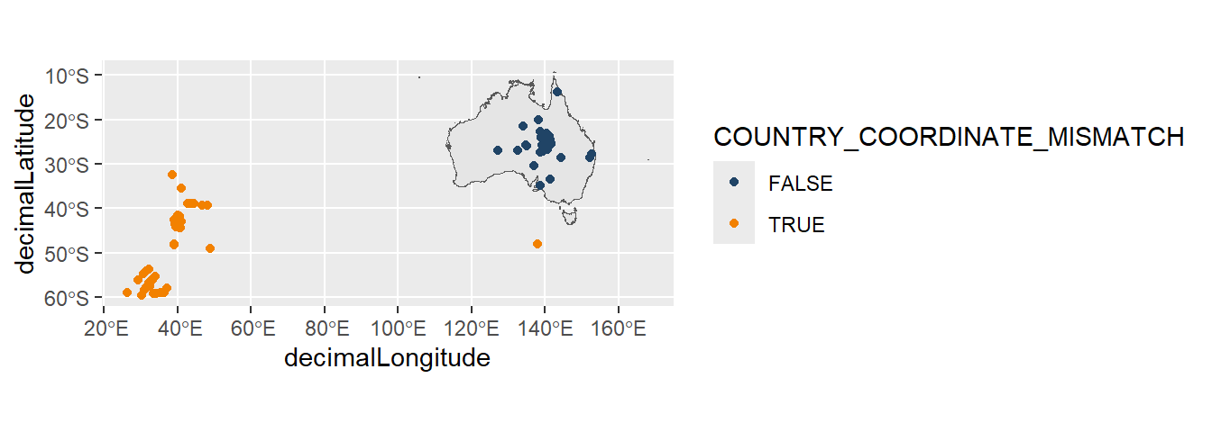
To remove these data, we can filter the dataset to exclude records that do not fall within Australia’s minimum and maximum coordinates.
native_mice_filtered <- native_mice |>
  filter(decimalLongitude > 100,
         decimalLongitude < 155,
         decimalLatitude > -45,
         decimalLatitude < -10)

ggplot() +
  geom_sf(data = aus) +
  geom_point(data = native_mice_filtered,
             aes(x = decimalLongitude,
                 y = decimalLatitude,
             colour = COUNTRY_COORDINATE_MISMATCH)) +
  pilot::scale_color_pilot()
10.3.2 Zero coordinates
Sometimes latitude and/or longitude data are recorded as having zero values; these values are not accurate representations of locations and thus should be removed.
Let’s use acacia data as an example. Including the ZERO_COORDINATE assertion column to your download allows us to identify records flagged as having zero values in the coordinate fields.
acacias <- acacias |>
  drop_na(decimalLatitude, decimalLongitude) # remove NA values

acacias |>
  select(ZERO_COORDINATE, everything())
# A tibble: 11,326 × 11
ZERO_COORDINATE recordID scientificName taxonConceptID decimalLatitude
<lgl> <chr> <chr> <chr> <dbl>
1 FALSE 00197d65-f235-… Acacia aneura https://id.bi… -29.5
2 FALSE 001a3cbb-a370-… Acacia aneura… https://id.bi… -28.0
3 FALSE 00238db7-6c4e-… Acacia aneura… https://id.bi… -34.1
4 FALSE 00276566-b590-… Acacia aneura https://id.bi… -29.7
5 FALSE 0029f3cf-b541-… Acacia aneura https://id.bi… -29.0
6 FALSE 0034f771-a3e1-… Acacia aneura https://id.bi… -31.1
7 FALSE 0035cb4f-85e5-… Acacia aneura… https://id.bi… -29.5
8 FALSE 003cce3b-f3f8-… Acacia aneura https://id.bi… -29.1
9 FALSE 0049bcbb-c8c2-… Acacia aneura https://id.bi… -25.5
10 FALSE 004dfec5-7095-… Acacia aneura https://id.bi… -28.6
# ℹ 11,316 more rows
# ℹ 6 more variables: decimalLongitude <dbl>, eventDate <dttm>,
# occurrenceStatus <chr>, dataResourceName <chr>, countryCode <chr>,
# locality <chr>We can see the flagged record in orange on our map.
ggplot() +
  geom_sf(data = aus) +
  geom_point(data = acacias,
             aes(x = decimalLongitude,
                 y = decimalLatitude,
                 colour = ZERO_COORDINATE)) +
  pilot::scale_color_pilot()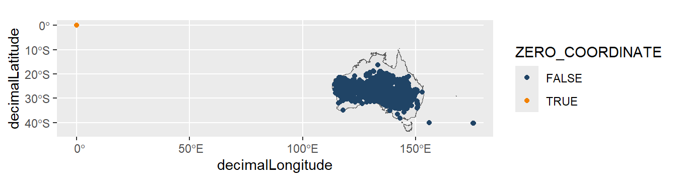
We can remove this record by filtering our dataset to remove records with longitude or latitude coordinates that equal zero.
acacias_filtered <- acacias |>
  filter(decimalLongitude != 0,
         decimalLatitude != 0)

ggplot() +
  geom_sf(data = aus) +
  geom_point(data = acacias_filtered,
             aes(x = decimalLongitude,
                 y = decimalLatitude,
                 colour = ZERO_COORDINATE)) +
  pilot::scale_color_pilot()
10.3.3 Centroids
Centroids, or coordinates that mark the exact centre point of an area, are sometimes assigned to an occurrence record when the original observation location was provided as a description. If a record was collected using a vague locality description or through incorrect geo-referencing, centroids can be used to categorise the record into broadly the correct area1.
Let’s use common brown butterfly data for our example.
WarningALA centroid assertions currently under review
The ALA is currently (September 2025) in the process of reviewing the COORDINATES_CENTRE_OF_COUNTRY and COORDINATES_CENTRE_OF_STATEPROVINCE assertions columns to ensure they are accurate. While this process is ongoing, we suggest using an alternative method of generating centroids for a map or polygon like sf::st_centroid() and comparing the coordinates to observation coordinates in your dataset.
Including the COORDINATES_CENTRE_OF_COUNTRY and/or COORDINATES_CENTRE_OF_STATEPROVINCE assertions columns to your download allows us to identify records flagged as containing centroid coordinates.
butterflies <- butterflies |>
  drop_na(decimalLatitude, decimalLongitude) # remove NA values

butterflies |>
  select(COORDINATES_CENTRE_OF_COUNTRY,
         COORDINATES_CENTRE_OF_STATEPROVINCE,
         everything())
# A tibble: 343 × 12
COORDINATES_CENTRE_OF_COUNTRY COORDINATES_CENTRE_OF…¹ recordID scientificName
<lgl> <lgl> <chr> <chr>
1 FALSE FALSE 018f5a5… Heteronympha …
2 FALSE FALSE 02eef43… Heteronympha …
3 FALSE FALSE 03b39bb… Heteronympha …
4 FALSE FALSE 04c2ac2… Heteronympha …
5 FALSE FALSE 05cced1… Heteronympha …
6 FALSE FALSE 05ceb8b… Heteronympha …
7 FALSE FALSE 06679b8… Heteronympha …
8 FALSE FALSE 0704e7b… Heteronympha …
9 FALSE FALSE 0756bd4… Heteronympha …
10 FALSE FALSE 0774f2e… Heteronympha …
# ℹ 333 more rows
# ℹ abbreviated name: ¹COORDINATES_CENTRE_OF_STATEPROVINCE
# ℹ 8 more variables: taxonConceptID <chr>, decimalLatitude <dbl>,
# decimalLongitude <dbl>, eventDate <dttm>, occurrenceStatus <chr>,
# dataResourceName <chr>, countryCode <chr>, locality <chr>Filtering our data to flagged records, we return one record.
butterflies |>
  filter(
    COORDINATES_CENTRE_OF_COUNTRY == TRUE |
    COORDINATES_CENTRE_OF_STATEPROVINCE == TRUE
    )
# A tibble: 1 × 12
recordID scientificName taxonConceptID decimalLatitude decimalLongitude
<chr> <chr> <chr> <dbl> <dbl>
1 89186e67-be72-… Heteronympha … https://biodi… -31.3 147.
# ℹ 7 more variables: eventDate <dttm>, occurrenceStatus <chr>,
# dataResourceName <chr>, countryCode <chr>, locality <chr>,
# COORDINATES_CENTRE_OF_COUNTRY <lgl>,
# COORDINATES_CENTRE_OF_STATEPROVINCE <lgl>The flagged record is the single orange point on our map.
ggplot() +
  geom_sf(data = aus) +
  geom_point(data = butterflies,
             aes(x = decimalLongitude,
                 y = decimalLatitude,
                 colour = COORDINATES_CENTRE_OF_STATEPROVINCE)) +
  pilot::scale_color_pilot() +
  theme(legend.position = "none")
We can remove this data point by excluding this record from our dataset.
butterflies_filtered <- butterflies |>
  filter(COORDINATES_CENTRE_OF_STATEPROVINCE == FALSE)

ggplot() +
  geom_sf(data = aus) +
  geom_point(data = butterflies_filtered,
             aes(x = decimalLongitude,
                 y = decimalLatitude,
                 colour = COORDINATES_CENTRE_OF_STATEPROVINCE)) +
  pilot::scale_color_pilot() +
  theme(legend.position = "none")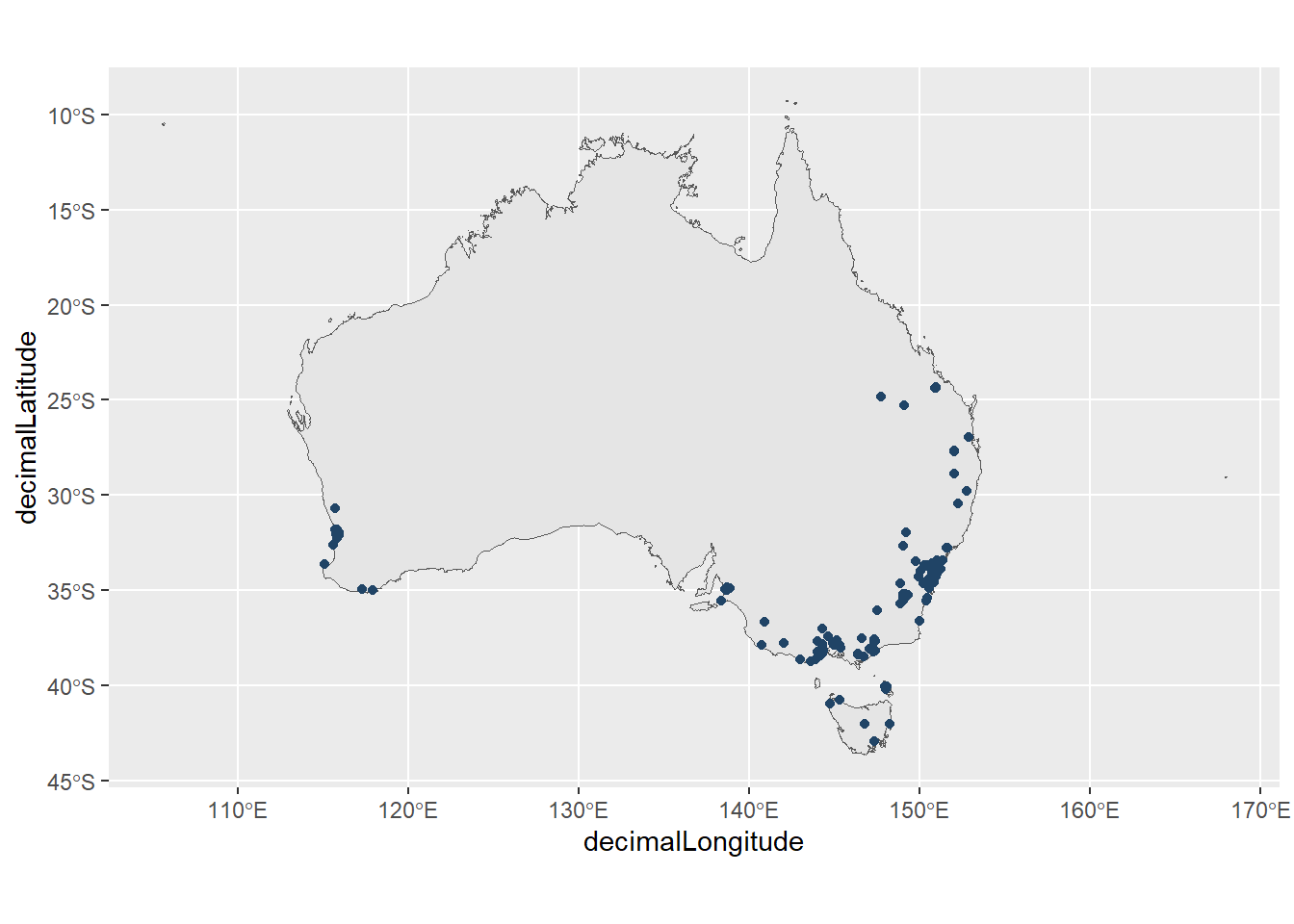
Keep in mind that just because an observation’s coordinates match a centroid doesn’t mean that the observation’s location is generalised (i.e., made less precise) to the centre of a polygon area. It could be coincidence! If you want to preserve as much data as possible, using other information can help determine if an observation’s coordinate location has been generalised or not. For example, the dataGeneralizations, coordinateUncertaintyInMetres and locality fields may offer extra context about whether an observation has been generalised because it is a sensitive record, or whether there is a location that the observation is more broadly associated with.
10.3.4 Cities, zoos, aquariums, museums & herbaria
Some observations are recorded in locations where animals and plants live but do not naturally occur. A common example is observations recorded at public facilities like zoos, aquariums, and botanic gardens.
Other times, observations are recorded in places where specimens of animals and plants might be stored, but not where they were observed. Common examples are museums and herbaria.
In some cases, like with records of the Gorse Bitter-pea, these locations can appear suspicious but not overly obvious. When we map these observations, there is a tailing distribution of points in Western Australia with several points located near the west coast of Australia.
bitter_peas <- bitter_peas |>
  drop_na(decimalLongitude, decimalLatitude) # remove NA values

ggplot() +
  geom_sf(data = aus) +
  geom_point(data = bitter_peas,
             aes(x = decimalLongitude,
                 y = decimalLatitude),
             colour = "#204466")
Suspiciously, if we Google the coordinates of the Western Australia Herbarium, the coordinates overlap with one of the points. We have highlighted this point in orange.
ggplot() +
  geom_sf(data = aus) +
  geom_point(data = bitter_peas,
             aes(x = decimalLongitude,
                 y = decimalLatitude),
             colour = "#204466") +
  geom_point(aes(x = 115.8, y = -31.9), # point coordinates
             colour = "#f28100") +
  theme(legend.position = "none")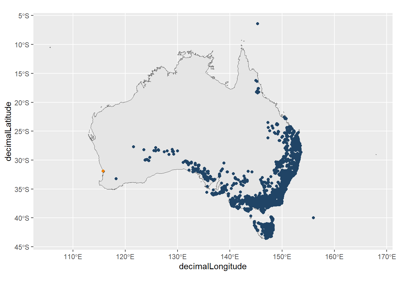
Filtering our data to the two left-most data points reveals that the data resources that supplied those records are both state herbaria.
bitter_peas |>
  filter(decimalLongitude < 120) |>
  select(dataResourceName)
# A tibble: 3 × 1
dataResourceName
<chr>
1 MBM herbarium - Museu Botânico Municipal - Herbário Virtual REFLORA
2 National Herbarium of Victoria (MEL) AVH data
3 NSW AVH feed Having identified this, these records can now be removed from our dataset.
bitter_peas_filtered <- bitter_peas |>
  filter(decimalLongitude > 120)

ggplot() +
  geom_sf(data = aus) +
  geom_point(data = bitter_peas_filtered,
             aes(x = decimalLongitude,
                 y = decimalLatitude),
             colour = "#204466")
TipUse
basisOfRecord
You can use the field basisOfRecord to avoid including records from museums and herbaria when creating your query in galah.
library(galah)

# Show values in `basisOfRecord` field
search_all(fields, "basisOfRecord") |>
  show_values()

# Filter basis of record to only human observations
galah_call() |>
  identify("Daviesia ulicifolia") |>
  filter(basisOfRecord == "HUMAN_OBSERVATION") |>
  atlas_counts()
10.4 Packages
Other packages exist to make identifying and cleaning geospatial coordinates more streamlined. The advantage of using these packages is that they can run many checks over coordinates at one time, rather than identifying each error separately like we did over this chapter. This process can make finding possible spatial outliers faster. The disadvantage is that checks might be more difficult to tweak compared to manual checks. Manual checks can also make the steps you made to clean your data clearer (and easier to edit later) in a complete data cleaning workflow.
Choose the package (or mix of packages and functions) that work best for you and your data cleaning needs.
CoordinateCleaner
The CoordinateCleaner package is a package for automated flagging of common spatial and temporal errors of biological and palaentological data. It is particularly useful for cleaning data from GBIF.
Here is an example of a general cleaning function, but there are many more bespoke options that the package offers.
library(CoordinateCleaner)

# Run record-level tests
coordinate_tests <- clean_coordinates(x = butterflies,
                                      species = "scientificName")
summary(coordinate_tests)
.val .equ .zer .cap .cen .sea .otl .gbf
0 0 0 22 0 11 60 0
.inst .summary
13 100 plot(coordinate_tests)
10.5 Summary
Each of the cleaning steps in this chapter do not have to be run in order, or even at all. Whether they are used is context- and taxon-dependent. As an example, what is one species that has many “wrong” coordinates based on many of the steps listed above?
The Great White Shark.

Code
# Download occurrence records
sharks <- galah_call() |>
  identify("Carcharodon carcharias") |>
  filter(basisOfRecord == "HUMAN_OBSERVATION") |>
  apply_profile(ALA) |>
  atlas_occurrences()

# Retrieve map of Australia
aus <- st_transform(ozmap_country, 4326)

# Map occurrences
sharks |>
  drop_na(decimalLongitude, decimalLatitude) |>
  ggplot() +
  geom_sf(data = aus,
          colour = "grey60",
          fill = "white") +
  geom_point(data = sharks,
             aes(x = decimalLongitude,
                 y = decimalLatitude),
             colour = "#135277") +
  theme_light()
The difficulty with cleaning Great White Shark occurrence data is that these sharks have a massive habitat range, and these locations along (what appear to be) the North American coast and Madagascar could very well be true occurrences. Be sure to consider the taxonomic and spatial range of your species before jumping into data cleaning!
This can happen when record locations are incorrectly given as the physical location of the specimen, or because they represent individuals from captivity or grown in horticulture (but were not clearly labelled as such).↩︎