# packages
library(galah)
library(dplyr)
galah_config(email = "your-email-here") # ALA-registered email

banksia <- galah_call() |>
  filter(doi == "https://doi.org/10.26197/ala.0deb6b7b-8899-4087-a4ff-e00340f53d6b") |>
  atlas_occurrences()

quokkas <- galah_call() |>
  filter(doi == "https://doi.org/10.26197/ala.229bac8f-ec80-4729-8bf4-0e0434a89fe5") |>
atlas_occurrences()9 Geospatial investigation
An important part of observational data is their location, specifying where each observation of an organism or species took place. These locations can range from locality descriptions (e.g., “Near Tellera Hill station”) to exact longitude and latitude coordinates tracked by a GPS system. The accuracy of these geospatial data will determine what types of ecological analyses you can use the data for. It is important to know how precise observations are, along with the range of uncertainty around an observation’s location, to contextualise any findings or conclusions made using the data.
In this chapter, we will discuss some different ways to assess the precision and uncertainty of occurrence record coordinates and highlight how to look for spatial characteristics or errors when visualising occurrences with maps.
9.0.1 Prerequisites
In this chapter we’ll use data of Banksia serrata occurrence records since 2022 and quokka occurrence records from the ALA.
To check data quality, data infrastructures like the Atlas of Living Australia have assertions—columns that data infrastructures use to flag when a record has an issue that fails a data cleaning check. If we use galah to download records, we can use assertions columns in our query to help identify and clean suspicious records.
If you would like to view assertions, use show_all().
assertions <- show_all(assertions)
assertions |>
  print(n = 7)
# A tibble: 124 × 4
id description category type
<chr> <chr> <chr> <chr>
1 AMBIGUOUS_COLLECTION Ambiguous collection Comment assertio…
2 AMBIGUOUS_INSTITUTION Ambiguous institution Comment assertio…
3 BASIS_OF_RECORD_INVALID Basis of record badly formed Warning assertio…
4 biosecurityIssue Biosecurity issue Error assertio…
5 COLLECTION_MATCH_FUZZY Collection match fuzzy Comment assertio…
6 COLLECTION_MATCH_NONE Collection not matched Comment assertio…
7 CONTINENT_COORDINATE_MISMATCH continent coordinate mismatch Warning assertio…
# ℹ 117 more rowsYou can use the stringr package to search for text matches.
assertions |>
  filter(str_detect(id, "COORDINATE")) |>
  print(n = 5)
# A tibble: 17 × 4
id description category type
<chr> <chr> <chr> <chr>
1 CONTINENT_COORDINATE_MISMATCH continent coordinate mismat… Warning asse…
2 CONTINENT_DERIVED_FROM_COORDINATES Continent derived from coor… Warning asse…
3 COORDINATE_INVALID Coordinate invalid Warning asse…
4 COORDINATE_OUT_OF_RANGE Coordinates are out of rang… Warning asse…
5 COORDINATE_PRECISION_INVALID Coordinate precision invalid Warning asse…
# ℹ 12 more rowsOver this chapter, we will detail when an assertion column can help identify occurrence records with geospatial issues.
9.1 Quick visualisation
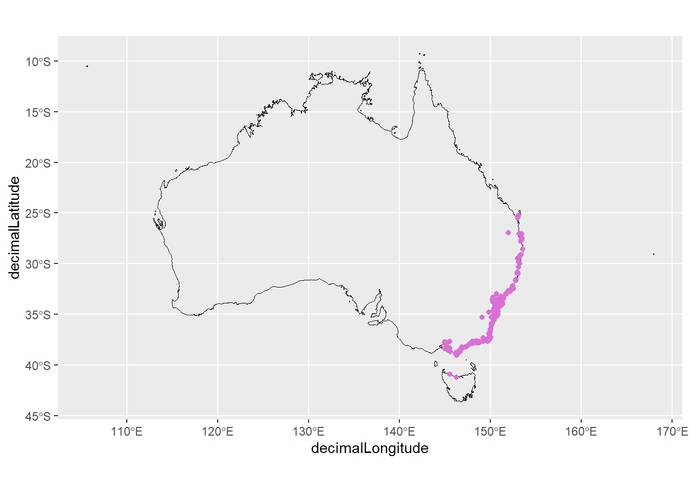
Mentioned in the Inspect chapter, one of the most straightforward ways to check for spatial errors is to plot your data onto a map. More obvious spatial errors are much easier to spot visually.
In most spatial datasets, the most important columns are decimalLatitude and decimalLongitude (or similarly named columns). These contain the latitude and longitude of each observation in decimal form (rather than degrees).
# Retrieve map of Australia
aus <- st_transform(ozmap_country, 4326)

# A quick plot of banksia occurrences
ggplot() +
  geom_sf(data = aus, colour = "black", fill = NA) +
  geom_point(data = banksia,
             aes(x = decimalLongitude,
                 y = decimalLatitude),
             colour = "orchid")
Warning: Removed 1 row containing missing values or values outside the scale range
(`geom_point()`).
9.2 Precision
Not all observations have the same degree of precision. Coordinate precision can vary between data sources and recording equipment. For example, coordinates recorded with a GPS unit or a phone generally have higher precision than coordinates recorded manually from a locality description.
The degree of precision you require will depend on the granularity of your research question and analysis. A fine-scale question will require data measured at a fine-scale to answer it. National or global scale questions require less precise data.
When downloading data from the ALA with the galah package, it’s possible to include the column coordinatePrecision—a decimal representation of how precise the coordinates of an observation are—to your data.
banksia |>
select(scientificName,
coordinatePrecision
) |>
filter(!is.na(coordinatePrecision))- 1
-
Not all records have this information recorded, so we also filter to only records with a
coordinatePrecisionvalue.
# A tibble: 82 × 2
   scientificName  coordinatePrecision
   <chr>                         <dbl>
 1 Banksia serrata         0.000000001
 2 Banksia serrata         0.000000001
 3 Banksia serrata         0.000000001
 4 Banksia serrata         0.000000001
 5 Banksia serrata         0.000000001
 6 Banksia serrata         0.000000001
 7 Banksia serrata         0.000000001
 8 Banksia serrata         0.000000001
 9 Banksia serrata         0.000000001
10 Banksia serrata         0.000000001
# ℹ 72 more rows
Only a few records have coordinatePrecision recorded, but that subset of records are very precise.
banksia |>
  group_by(coordinatePrecision) |>
  count()
# A tibble: 2 × 2
# Groups: coordinatePrecision [2]
coordinatePrecision n
<dbl> <int>
1 0.000000001 82
2 NA 727Filter your records to only those under a specific measure of precision.
# Filter by number of decimal places
banksia <- banksia |>
  filter(coordinatePrecision <= 0.001)
9.3 Uncertainty
Similarly, not all observations have the same degree of location certainty. An organism’s exact location will likely have an area of uncertainty around it, which can grow or shrink depending on the method of observation and the species observed. For example, if a person uses a precise GPS and high-definition camera to make observations of snails, their observed location will be of higher certainty than a person using a phone camera to make observations of birds in the distance. The exact location might also be obscured for sensitivity purposes. Uncertainty inevitably affects how robust the results from species distribution models are.
When downloading data from the ALA with the galah package, it’s possible to include the column coordinateUncertaintyInMeters—a measure of the circular area that captures the true location—to your data. We added this column in our original galah query.
banksia |>
  select(scientificName,
         coordinateUncertaintyInMeters
         )
# A tibble: 809 × 2
scientificName coordinateUncertaintyInMeters
<chr> <dbl>
1 Banksia serrata 316
2 Banksia serrata 2268
3 Banksia serrata NA
4 Banksia serrata NA
5 Banksia serrata NA
6 Banksia serrata 15
7 Banksia serrata 4
8 Banksia serrata NA
9 Banksia serrata NA
10 Banksia serrata 2457
# ℹ 799 more rowsThere is a range of coordinate uncertainty in our data, with many falling within 10m of uncertainty.
banksia |>
  group_by(coordinateUncertaintyInMeters) |>
  count()
# A tibble: 155 × 2
# Groups: coordinateUncertaintyInMeters [155]
coordinateUncertaintyInMeters n
<dbl> <int>
1 1 4
2 2 6
3 3 35
4 4 139
5 5 59
6 6 18
7 7 14
8 8 27
9 9 19
10 10 70
# ℹ 145 more rowsIf your analysis requires greater certainty, you can then filter your records to a smaller area of uncertainty.
# Filter by number of decimal places
banksia <- banksia |>
  filter(coordinateUncertaintyInMeters <= 5)
9.4 Obscured location
Occurrence records of sensitive, endangered or critically endangered species my be obscured (i.e. generalised, obfuscated) to protect the true location of the species. This process blurs the of an organism actual location to avoid risks like poaching or capture while still allowing their data to be included in broader summaries.
In the ALA, the field dataGeneralizations contains information of whether a record has been has been obscured and the size of the area the point has been generalised to.
dataGeneralizations
The dataGeneralizations field will only be available to use or download when there are records in your query that have been generalised/obscured.
search_all(fields, "dataGeneralization")# A tibble: 2 × 3
id description type
<chr> <chr> <chr>
1 dataGeneralizations Data Generalised during processing fields
2 raw_dataGeneralizations <NA> fieldsFor example, the Western Swamp Tortoise is a critically endangered species in Western Australia. There are 97 total observations of this species in the ALA.
galah_call() |>
  identify("Pseudemydura umbrina") |>
  atlas_counts()
# A tibble: 1 × 1
count
<int>
1 127Grouping record counts by the dataGeneralizations column shows that 96 of the 97 records have been obscured by 10 km.
galah_call() |>
  identify("Pseudemydura umbrina") |>
  group_by(dataGeneralizations) |>
  atlas_counts()
# A tibble: 1 × 2
dataGeneralizations count
<chr> <int>
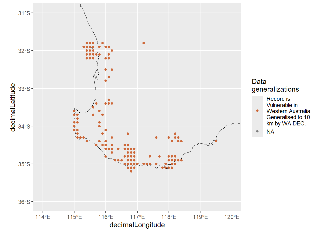
1 Record is Critically Endangered in Western Australia. Generalised to 10… 126What do obscured data look like?
Quokka data offer a nice example to get an idea of what to look for when data points have been obscured. When plotted, obscured occurrence data appears as if points were plotted onto a grid 1.
# remove records with missing coordinates
quokkas <- quokkas |>
  tidyr::drop_na(decimalLatitude, decimalLongitude)

# aus map
aus <- ozmap_country |> st_transform(4326)

# map quokka occurrences
ggplot() +
  geom_sf(data = aus, colour = "black", fill = NA) +
  geom_point(data = quokkas,
             aes(x = decimalLongitude,
                 y = decimalLatitude,
                 colour = dataGeneralizations |>
                   str_wrap(18))) +
  scale_colour_manual(values = c("sienna3", "snow4"),
                      guide = guide_legend(position = "bottom")) +
  guides(colour = guide_legend(title = "Data\ngeneralizations")) +
  xlim(114,120) +
  ylim(-36,-31)
Warning: Removed 2 rows containing missing values or values outside the scale range
(`geom_point()`).
Keep in mind that survey data can also appear gridded if survey locations were dispersed at equal distance, so be sure to double check before assuming data has been obscured!
For more information, check out ALA’s support article about working with threatened, migratory and sensitive species.
9.5 Summary
In this chapter, we showed some ways to investigate the geospatial coordinates of your data and determine its level of precision, uncertainty or obscurity.
In the next chapter, we’ll see examples of issues with coordinates that require fixing or removing.
This is pretty much what actually happened—locations have been “snapped” onto a grid determined by the generalised distance.↩︎


